1.5 Preferences II: MRS and Marginal Utility - Class Notes
Contents
Thursday, January 30, 2020
Overview
We continue with our model of how individuals choose. Our focus for this class is to wrap up what we mean by “maximizing utility” as a person’s objective. We will do some practice problems on understanding indifference curves and utility functions. Then we will finally be ready to put our tools together next class to solve the consumer’s problem.
Slides
Practice Problems
Today you will be working on practice problems. Answers will be posted later.
Math Appendix
Graphing Indifference Curves
I will not ask you to formally graph indifference curves (just roughly sketch them where appropriate). If you wanted to graph them, and express them in a graphable (slope-intercept form) equation, simply solve for the good on the vertical axis.
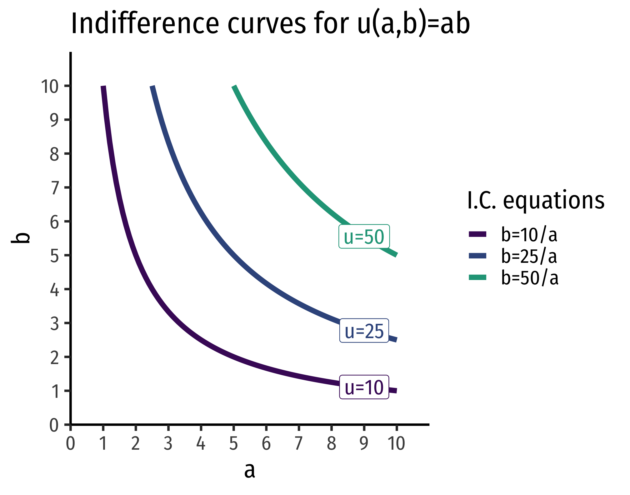
Example: Suppose we have a typicalCobb-Douglas!
indifference curve for apples \((a)\) and bananas \((b)\):
\[u(a,b)=ab\]
Each indifference curve (or contour) is one level of utility (all points on the curve give a specific level of utility). So, set that level of utility equal to some constant, \(k\).
\[ab=k\]
Then, if we are putting \(b\) on the vertical axis, we simply solve this for \(b\):
\[\begin{align*} ab&=k\\ b&=\frac{k}{a}\\ \end{align*}\]
This is the general equation for all indifference curves of this utility function: each utility level (value of \(k)\) can be graphed as an indifference curve with that equation. Thus, for example, for a utility level of \(10\), the equation for that indifference curve is \[b=\frac{10}{a}\].
Utility Functions for Perfect Substitutes
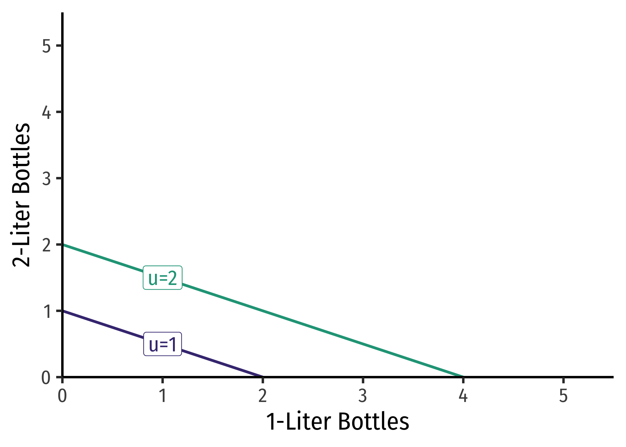
Perfect substitutes produce straight lines for indifference curves. A straight line has a constant slope, which is interpretted as the MRS being constant - you should always be willing to substitute between the two goods at the same rate. The utility function looks like:
\[u(x,y)=w_xx+w_yy\]
Where each \(w_i\) is a relative weight (intensity of relative preference). These are often known as linear preferences because the utility of the two goods are related by addition.
Notice, having some of one good and none of the other still provides positive utility (unlike utility functions where the quantities of goods are multiplied!). This is precisely because of the substitutability between the goods!
Example
Consider 1-Liter bottles of Coke \(L_{1}\) and 2-Liter bottles of Coke \(L_{2}\). You should always be willing to substitute between one 2-Liter bottle and two 1-Liter bottles.
\[u_{L_{1},L_{2}}=1L_{1}+2L_{2}\]
The relative weights here are 1 for 1-Liter bottles and 2 for 2-Liter bottles, because 2-Liter bottles are “worth” twice as much for you (it takes two 1-Liter bottles to match a 2-Liter bottle!).
\(MRS_{L_{1},L_{2}}=-\frac{w_x}{w_y} = -\frac{1}{2}\)
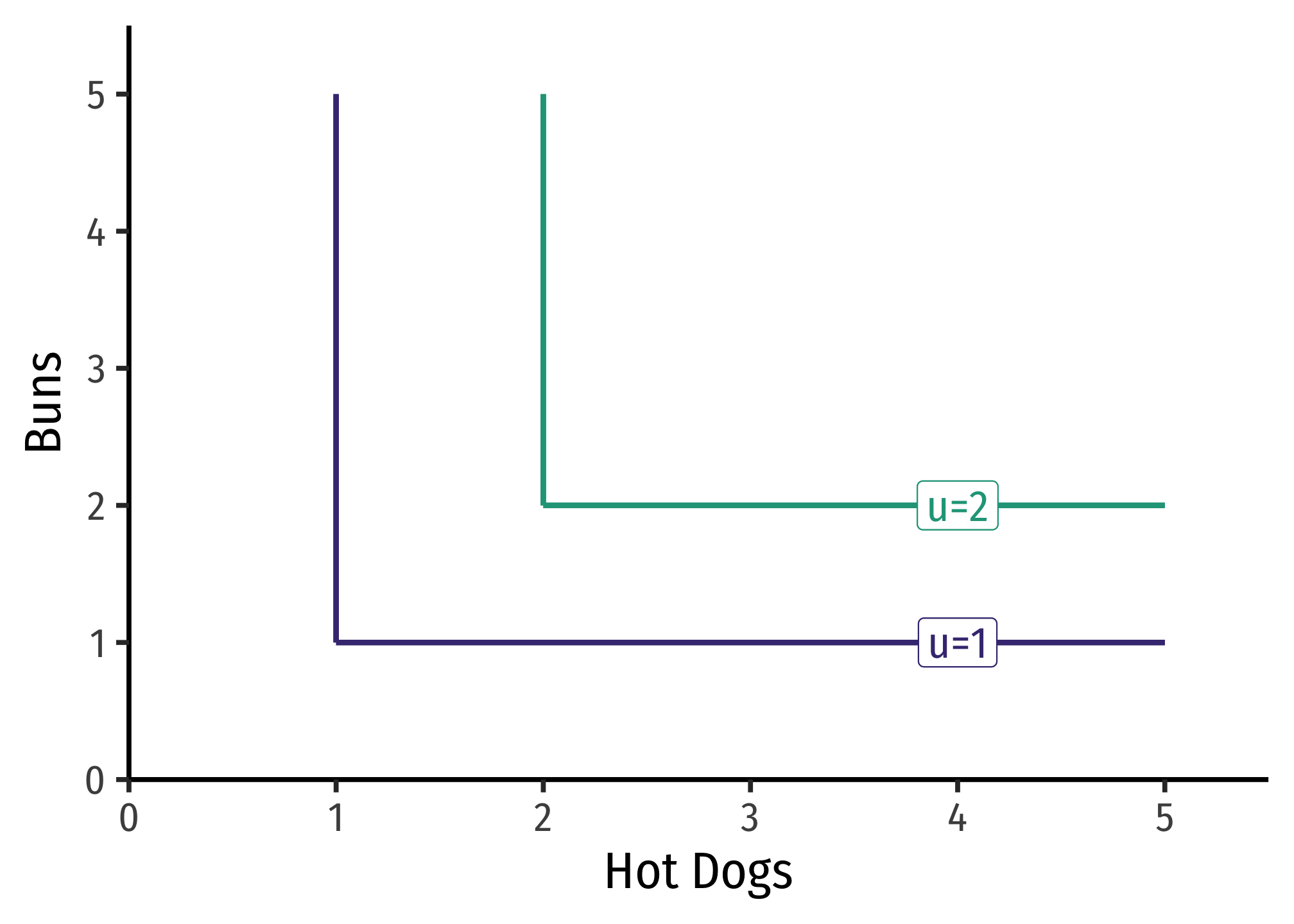
Utility Functions for Perfect Complements
Perfect complements produce right angles for indifference curves. This is technically not a mathematical function, since each \(X\) value must be mapped to a single \(Y\) value (i.e. no vertical lines). Thus, the utility function for perfect complements \(x\) and \(y\) is quite unique:
\[u(x,y)=min\{w_xx,w_yy\}\]
Where each \(w_i\) is a relative weight (intensity of relative preference). Utility is determined by the lesser value of what you have, \(x\) (weighted by \(w_x\)) or \(y\) (weighted by \(w_y\)). These are sometimes called “Leontief preferences”.
The marginal rate of substitution alternates between \(0\) (horizontal line) and \(\infty\) (vertical line).
Example
Consider consuming hot dogs \((H)\) and buns \((B)\), that must be consumed together as a package 1:1. The utility function would be: \[u(H,B)=min\{H,B\}\]
Having 2 hot dogs and 3 buns only yields a utility of 2. Having 3 hot dogs and 2 buns also only yields a utility of 2.
Cobb-Douglas Functions
Cobb-Douglas functions (both for utility and production) are one of the most common functional forms in economics. Despite their somewhat frightening presence on the surface, they have very neat mathematical properties, and have been empirically useful as well. A Cobb-Douglas function (for utility) looks like:
\[u(x, y)=x^a y^b\]
MRS and Positive Monotonic Transformations
The marginal rate of substitution, using the above equation is: \[\begin{align*} MRS_{x, y} &=\frac{MU_{x}}{MU_{y}} && \text{The definition of MRS}\\ &= \cfrac{\big(\frac{\partial }{\partial x}\big)}{\big(\frac{\partial}{\partial y}\big)} && \text{Using the definition of marginal utility as partial derivative}\\ &= \frac{a x^{a-1}y^b}{b x^a y^{b-1}} && \text{Differentiating }u \text{ w.r.t }x \text{ on top and }y \text{ on bottom}\\ &=\frac{a}{b} x^{(a-1)-a}y^{b-(b-1)} && \text{Using exponent rules for division}\\ &= \frac{a}{b} x^{-1}y^{1} && \text{Simplifying exponents}\\ &=\frac{a}{b} \frac{y}{x} && \text{Using exponent rules for negative exponents}\\ \end{align*}\]
Using logarithms, we can take a positive monotonic transformation of the original utility function \(u\):
\[v(x, y)=a \: ln \: x + b \: ln \: y\]
The MRS using the logarithmic form is:
\[\begin{align*} MRS_{x, y} &=\frac{MU_{x}}{MU_{y}} && \text{The definition of MRS}\\ &= \cfrac{\big(\frac{\partial }{\partial x}\big)}{\big(\frac{\partial}{\partial y}\big)} && \text{Using the definition of marginal utility as partial derivative}\\ &= \cfrac{\big(\frac{a}{x}\big)}{\big(\frac{b}{y}\big)} && \text{Differentiating }u \text{ w.r.t }x \text{ on top and }y \text{ on bottom}\\ &=\frac{a}{b} \frac{y}{x} && \text{Multiplying the righthand side by the reciprocal of the denominator,} \frac{y}{b}\\ \end{align*}\]
Which of course, is the same, because we know any positive monotonic transformation of a utility function preserves the same preferences!
EXAMPLE
Find the marginal rate of substitution for the utility function:
\[u(x, y) = \sqrt{x, y}\]
First, recognize that square roots are equivalent to saying \(x^{0.5} y^{0.5}\). The marginal rate of substitution would be:
\[\begin{align*} MRS_{x, y} &=\frac{MU_{x}}{MU_{y}} && \text{The definition of MRS}\\ &= \cfrac{\big(\frac{\partial }{\partial x}\big)}{\big(\frac{\partial}{\partial y}\big)} && \text{Using the definition of marginal utility as partial derivative}\\ &= \frac{0.5 x^{-0.5}y^{0.5}}{0.5x^{0.5}y^{-0.5}} && \text{Differentiating }u \text{ w.r.t }x \text{ on top and }y \text{ on bottom}\\ &=\frac{0.5}{0.5} x^{0.5-0.5}y^{0.5-(-0.5)} && \text{Using exponent rules for division}\\ &= x^{-1}y^{1} && \text{Simplifying exponents, and cancelling} \frac{0.5}{0.5}\\ &=\frac{y}{x} && \text{Using exponent rules for negative exponents}\\ \end{align*}\]
Note we could find this equivalently again by taking logs of the original utility function.
\[v(x,y)=0.5 \: ln \: x+0.5\: ln\: y\]
\[\begin{align*} MRS_{x, y} &=\frac{MU_{x}}{MU_{y}} && \text{The definition of MRS}\\ &= \cfrac{\big(\frac{\partial }{\partial x}\big)}{\big(\frac{\partial}{\partial y}\big)} && \text{Using the definition of marginal utility as partial derivative}\\ &= \cfrac{\big(\frac{0.5}{x}\big)}{\big(\frac{0.5}{y}\big)} && \text{Differentiating }u \text{ w.r.t }x \text{ on top and }y \text{ on bottom}\\ &=\frac{y}{x} && \text{Multiplying the righthand side by the reciprocal of the denominator,} \frac{y}{0.5}\\ \end{align*}\]
Which again, gives us the same marginal rate of substitution.