1.8 Income and Substitution Effects - Class Notes
Contents
Thursday, February 13, 2020
Overview
Today we cover the third effect: the (own) price effect, aka the law of demand: how changes in a good’s (own) price affect quantity demanded for that good. We introduce the idea of demand functions, inverse demand functions, and a demand curve. I will also show you examples of how we derive demand functions and curves.
The other major concept today is breaking apart the law of demand into two effects: the (real) income effect, and the substitution effect. We considering them conceptually and graphically. These can be a difficult concept for students to grasp.
Slides
Interactive Examples
- Visualizing the Consumer’s Problem
- Visualizing Changes in the Consumer’s Problem
- Visualizing Demand Shifters
These are examples that I wrote in R/Shiny in the past, to visualize what it is we are looking at. As I find more time, I will update these and integrate them into our slides, but until then, I will just post links.
The first is a visual example of the static (one-time) Consumer’s problem. You can adjust things about the (Cobb-Douglas) utility function, income, and prices, and see how it would affect the graph and the optimum.
The second is a visual example of dynamic changes in the Consumer’s problem. The consumer starts at a pre-defined optimum. You can adjust any of the budget constraint parameters (m,px,py), and see how it would affect a new optimum, which you can compare the the original optimum.
The third is a visual example of a hypothetical demand function for beer, with preference intensity, income, price of nachos (a complement), and price of wine (a substitute) as inputs to the function. Based on some pre-defined functions (in the background), you can change any of the inputs and see how it would affect the (inverse) demand function, expressed as a simple demand curve.
I hope some time to clean these up and make a few more, such as “Visualizing the Income and Substitution Effects” and “Estimating a Demand Function from Real World Data.”
Practice Problems
Answers to last class’ practice problems (on elasticities) are posted on that page. There are no official practice problems for today, but you should try to draw the full (real) income and substitution effects graph for a price change (for a normal good) on your own!
Assignments: Problem Set 1 is DUE and Problem Set 2
Problem set 1 is DUE!
Problem set 2 (on classes 1.7-1.9) is also posted, and is due by Thursday February 20. You will not be able to do everything on it until we complete class 1.9.
We will do a review day on Thursday, February 20. Expect Exam 1 to be on Tuesday, February 25.
Math Appendix
Example Demand Functions
The examples below show how we can take a utility function and derive a demand function.
Perfect Substitutes
Recall that perfect substitutes have indifference curves that are straight lines (constant MRS), and have a utility function of:
u(x,y)=w1x+w2y
Since both the budget constraint and the indifference curves are straight lines, we will not have a point of tangency between them, but a point(s) where the lines intersect.
There are three possible cases,
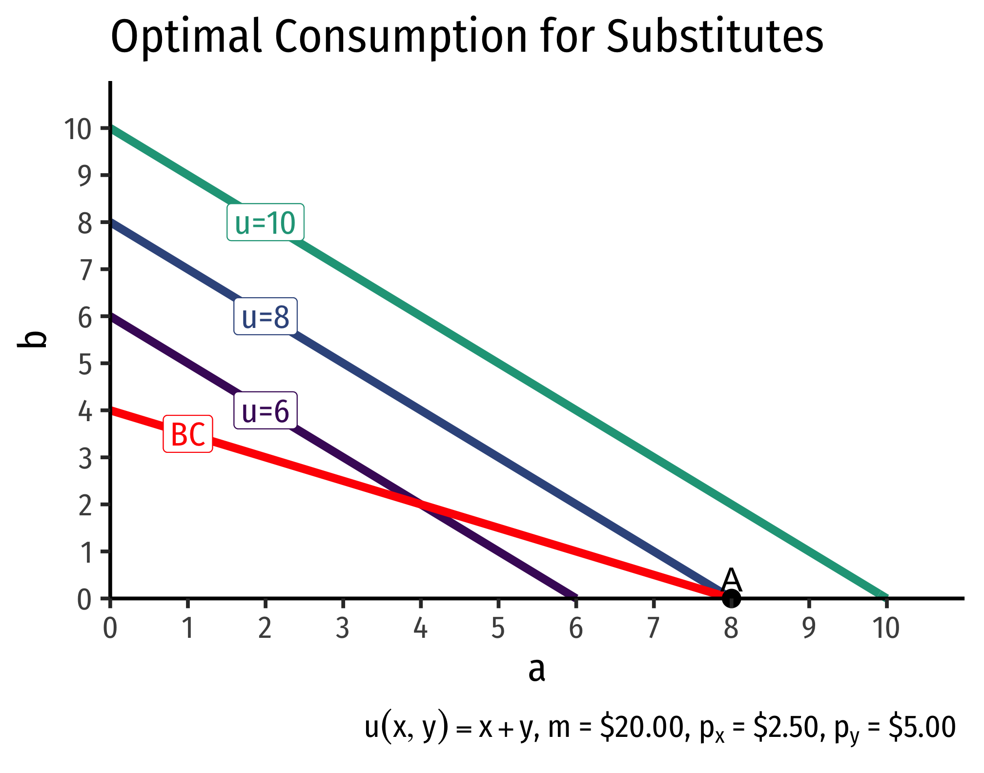
- if px>py, the slope of the budget constraint is flatter than the slope of the indifference “curves.” The optimal bundle is spending all income on good x.
- if px<py, the slope of the budget constraint is steeper than the slope of the indifference “curves.” The optimal bundle is spending all income on good y.
- if px=py, the budget constraint and indifference “curves” are the same line, so any point on the lines is optimal!
The first two cases are known as “corner solutions,” where a consumer chooses all of one good, and none of another. Note perfect substitutes are not convex, and violate the assumption that “averages are preferred to extremes.”
We can therefore write the demand function for good x (and similarly for y):
qxd={mpxWhen px<pyany number between 0 and mpxWhen px=py0When px>py
Perfect Complements
Recall that perfect complements have indifference curves that are right angles, and have a utility function of:
u(x,y)=min{w1x,w2y}
The optimal choice must always be at the corner of the indifference “curves.”
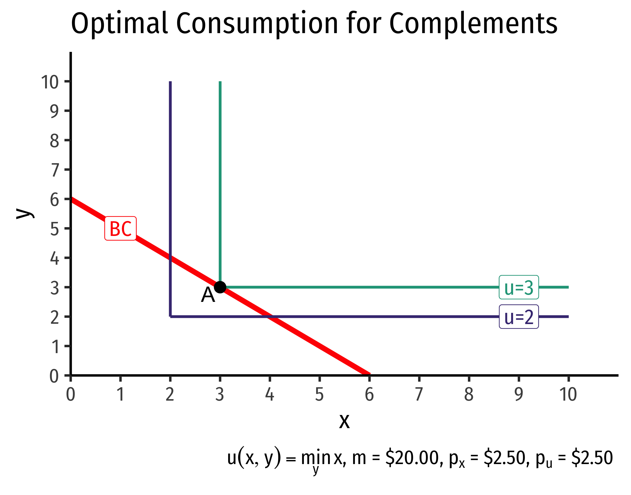
The consumer is purchasing equal amounts of x and y in this example, no matter what the prices are of either, so x=y. We must satisfy the budget constraint, that pxx+pyx=m (recall y=x). Solving this for x gives us the demand function for good x:
qxD=qyD=mpx+py
This should be intuitive: the consumer must always purchase equal amounts of x and y, so it’s as if the consumer was spending all of their income on a single good (x+y) that has a price of (px+py).
Cobb-Douglas
Now we come to a more realistic demand function. If a consumer has a Cobb-Douglas utility functionNote: Natural logs are easier to work with, this function is equivalent to u(x,y)=xayb.
u(x,y)=alnx+blny
Then we are solving the following constrained optimization problem:
maxx,yalnx+blny
I will solve this using the Lagrangian method.Note you could solve this by substitution. Use the definition of the optimum, that MUxMUy=pxpy, plug in, and solving carefully for x.
L=alnx+blny−λ(pxx+pyy−m)
The First Order Conditions are:
∂L∂x=ax−λpx=0∂L∂y=by−λpy=0∂L∂λ=pxx+pyy−m=0
Rearranging the first two FOCs:
a=λpxxb=λpyy
Adding them together:
a+b=λ(pxx+pyy)a+b=λm
Solving for λ:
λ=a+bm
Substitute this back into each of the first two FOCs and solve for x and y, respectively, to get:
x=aa+bmpxy=ba+bmpy
These are the demand functions for goods x and y. One of the convenient properties of Cobb-Douglas preferences is that a consumer spends a constant fraction of income (aa+b) on good x, and the complement fraction (ba+b) on good y!^This becomes especially simple when the exponents a+b=1, as in:
u(x,y)=xay(1−a)where 0 < a < 1
So a and 1−a are proportions of m!]
For a constant value of px, this is a linear function of m. So doubling, tripling, etc. m will double, triple, etc. quantity demanded for x. So the income expansion path (see previous class) is a straight line through the origin with a slope apx.
EXAMPLE
Suppose a consumer has a utility function
u(x,y)=x0.5y0.5
and faces constraints of m=50, pa=10, pb=5.
maxx,yx0.5y0.5
Write the Lagrangian (and taking logs of the objective function, for simplicity):
L=0.5lnx+0.5lny−λ(10x+5y−50)
FOCs are:
∂L∂x=0.5x−10λ=0∂L∂y=0.5y−5λ=0∂L∂λ=10x+5y−50=0
Rearrange the first two FOCs:
0.5=10λx0.5=5λy
Add then together, and solve for λ:
1=λ(10x+5y)1=λ(50)150=λ
Now substitute lambda into each of the first two FOCs, solving for x and y, respectively:
0.5x=10(150)10x=0.5(50)x=2.5
0.5y=5(150)10x=0.5(50)y=5
This consumer buys 2.5 units of x at $10/each ($25) and 5 units of y at $5/each ($25), spending all $50.
Recall the utility function is
u(x,y)=√xy=x0.5y0.5
Note the Cobb-Douglas exponents on x and y are equal and sum to 1: (a and 1−a=0.5). So the consumer spends a=50% of her income on x, and 1−a=50% on y.
To get the demand functions for x and y, go back to the FOCs, and keep all budget constraint terms as variables (px,py,m).
∂L∂x=0.5x−pxλ=0∂L∂y=0.5y−pyλ=0∂L∂λ=pxx+pyy−m=0
Rearrange the first two FOCs:
0.5=pxλa0.5=pyλy
Add then together, and solve for λ:
1=λ(pxx+pyy)1=λ(m)1m=λ
Substitute this back into each of the first two FOCs and solve for x, and y, respectively, to get:
0.5x−pxλ=00.5x−px(1m)=00.5x=pxmpxx=0.5mx=0.5mpx
0.5y−pyλ=00.5y−py(1m)=00.5y=pympyy=0.5my=0.5mpy
These are the demand functions for x and for y.Note you can just take the rule learned above, that x=ampx and y=bmpy and plug in a and b.
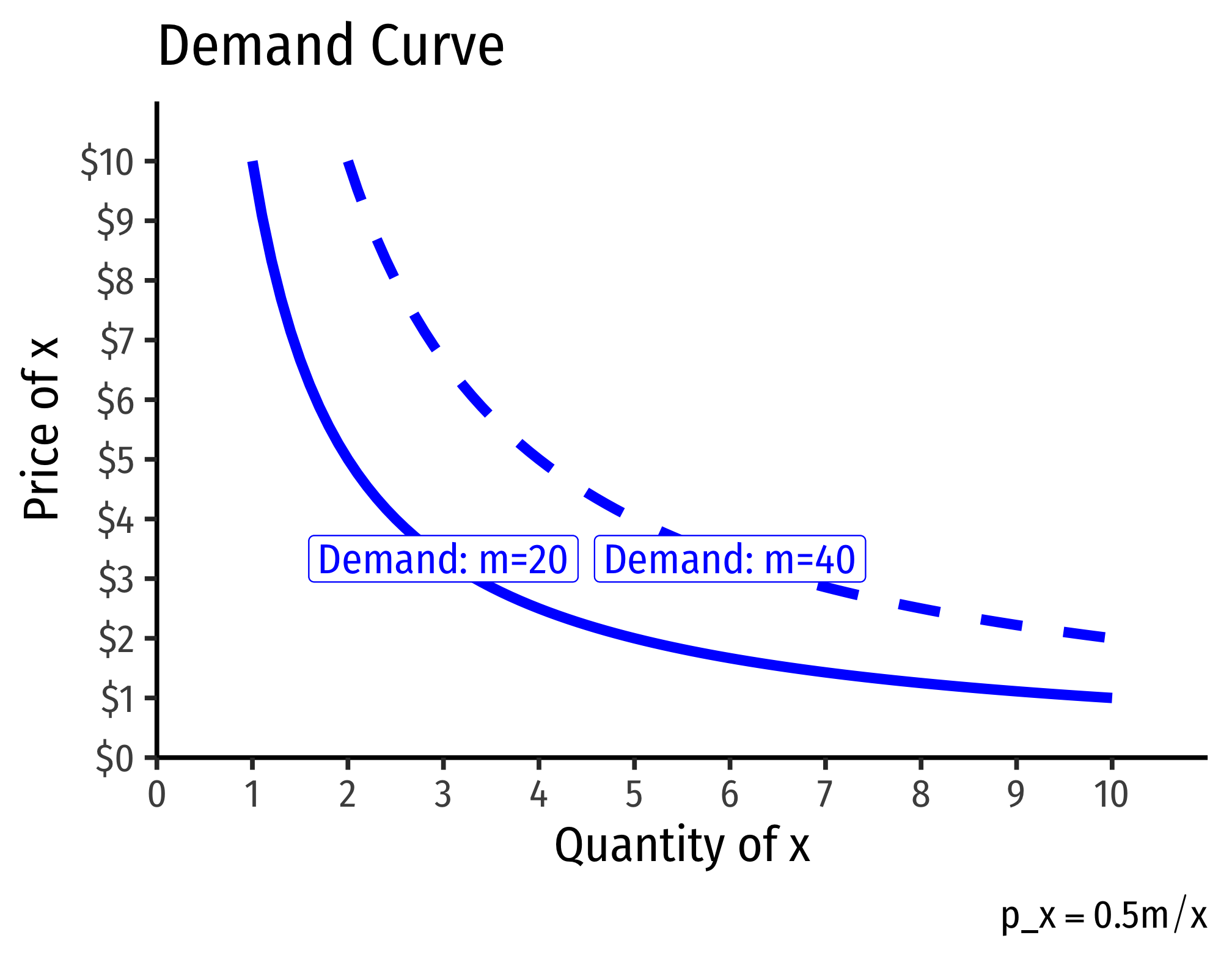
Note if we want to graph this, we need to find the inverse demand function by solving for px:
x=0.5mpxpxx=0.5mpx=0.5mx
Now we can graph a demand function for a given amount of income. As income changes, the demand curve shifts. Here are two examples, one where m=20 and another where m=40: