2.4 Costs of Production - Class Notes
Contents
- Tuesday, March 23, 2020
- Quarantine Lecture 1
Overview
Today we cover costs and revenues before we put them together next class to solve the firm’s profit maximization problem.
Class Livestream/Lecture Videos
See the above video for a brief overview of Zoom.
Slides
Assignments: Exam 1 Corrections & Homework 3
You will have until the end of the semester (May 4) to turn in your corrections, however, I advise you to do them as soon as possible. See more from the online transition page for details.
Homework 3 is now due, via email, on Sunday, March 29, by 11:59PM. The answer key will be posted Monday, March 30.
Appendix
The Relationship Between Returns to Scale and Costs
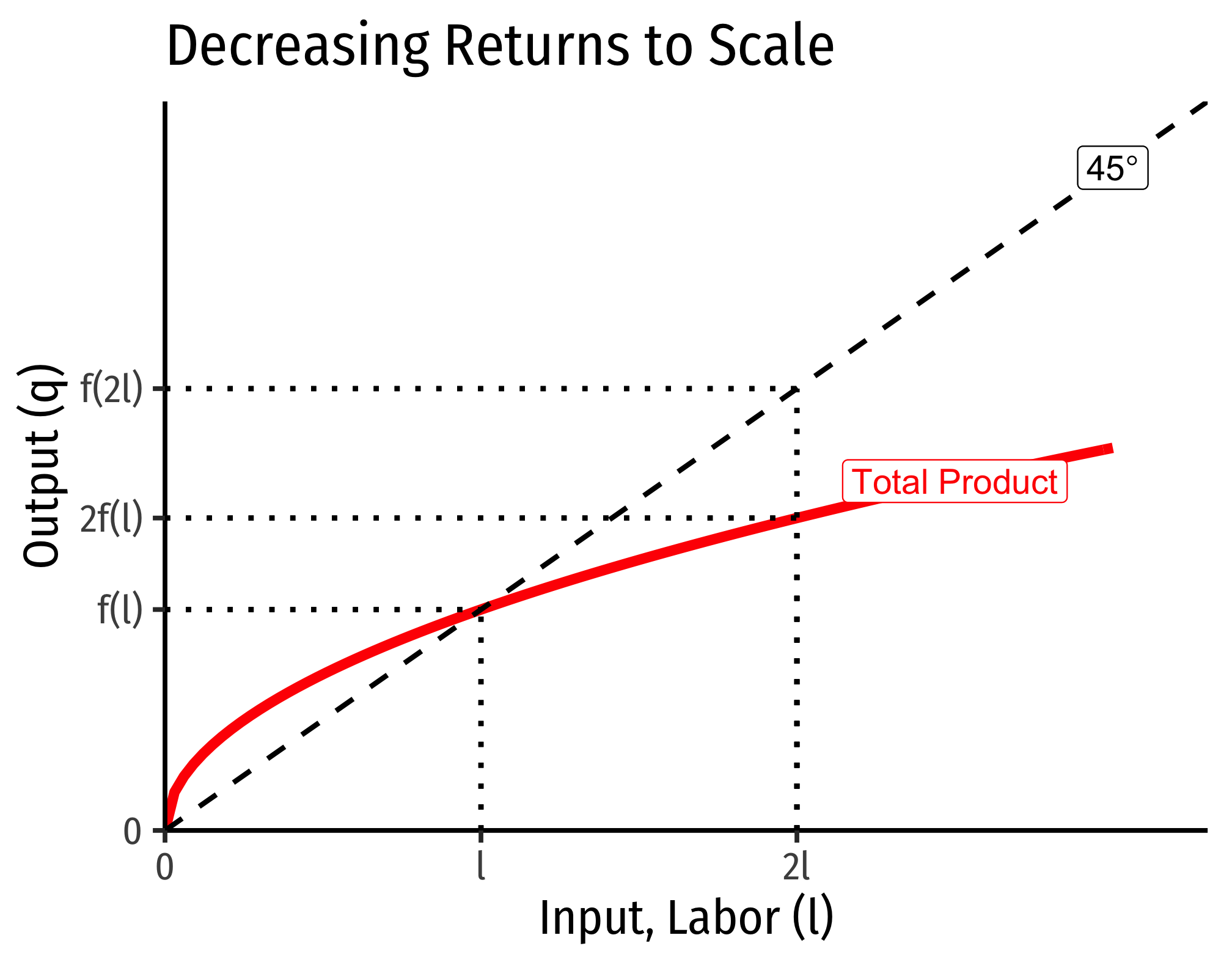
There is a direct relationship between a technology’s returns to scaleIncreasing, decreasing, or constant
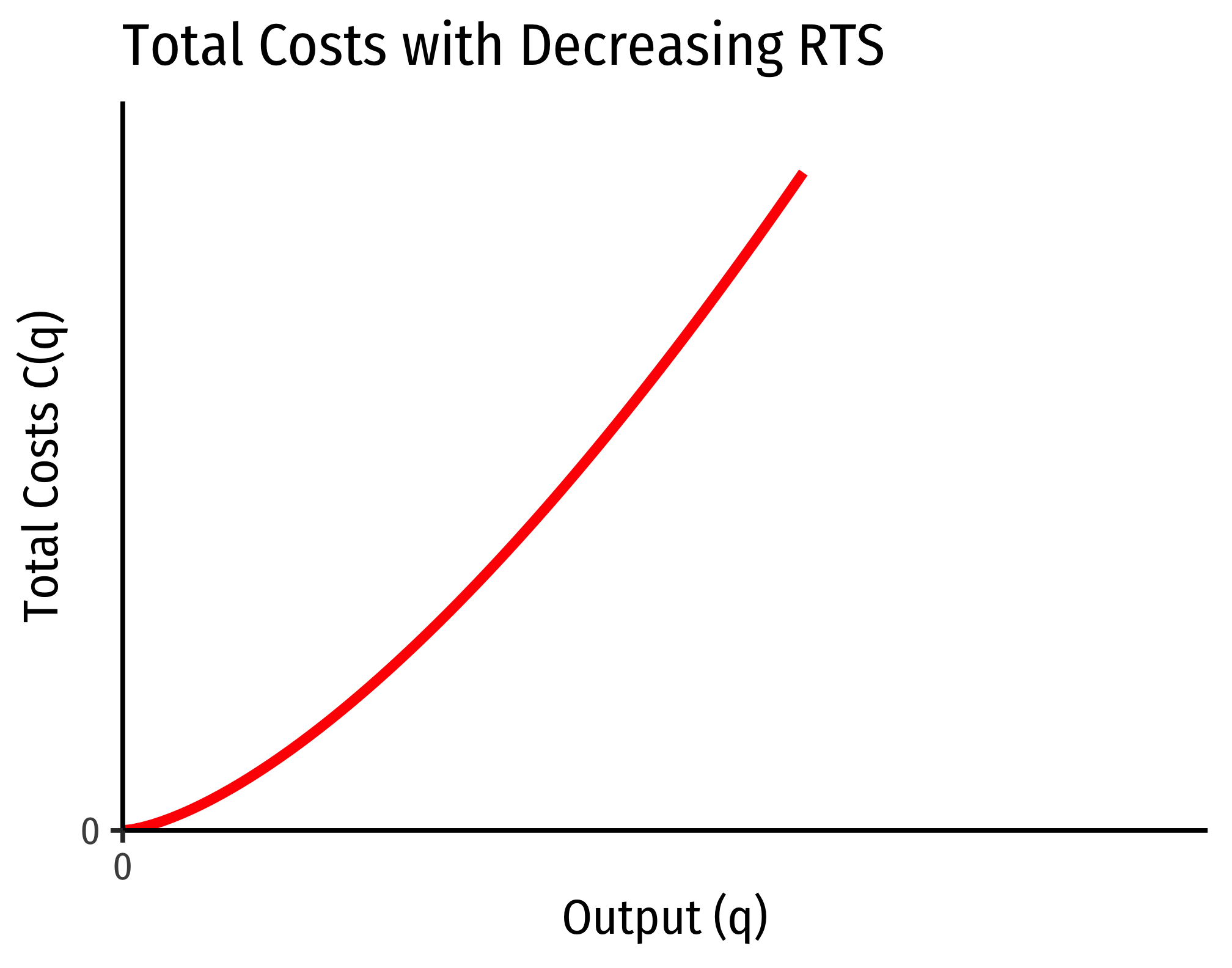
and its cost structure: the rate at which its total costs increaseAt a decreasing rate, at an increasing rate, or at a constant rate, respectively
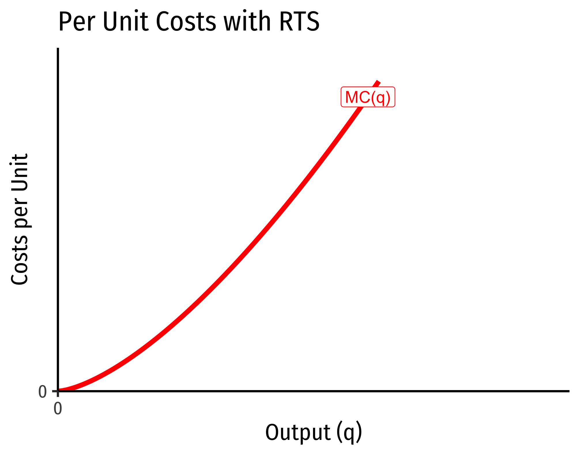
and its marginal costs changeDecreasing, increasing, or constant, respectively
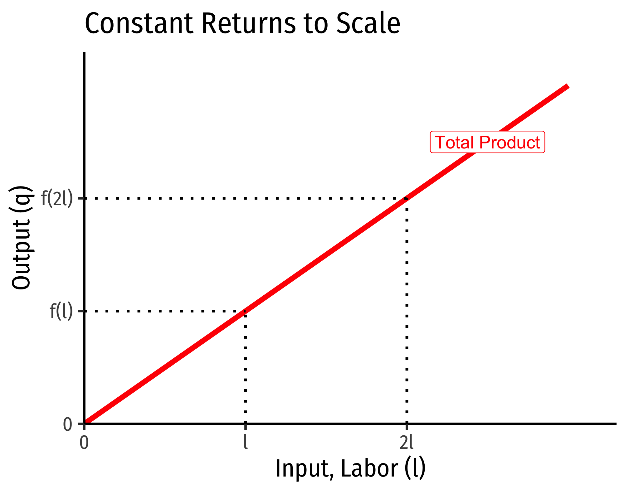
. This is easiest to see for a single input, such as our assumptions of the short run (where firms can change \(l\) but not \(\bar{k})\):
\[q=f(\bar{k},l)\]
Constant Returns to Scale:
Decreasing Returns to Scale
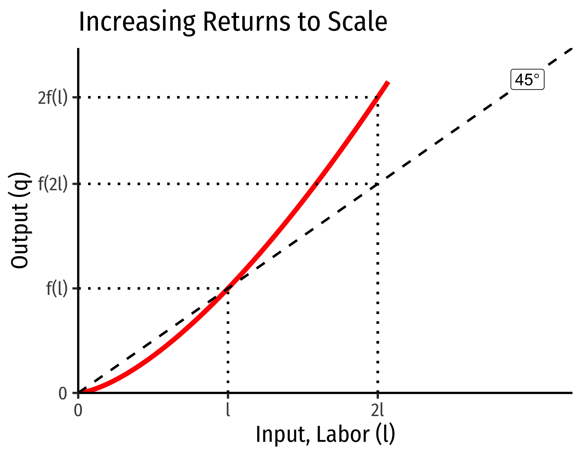
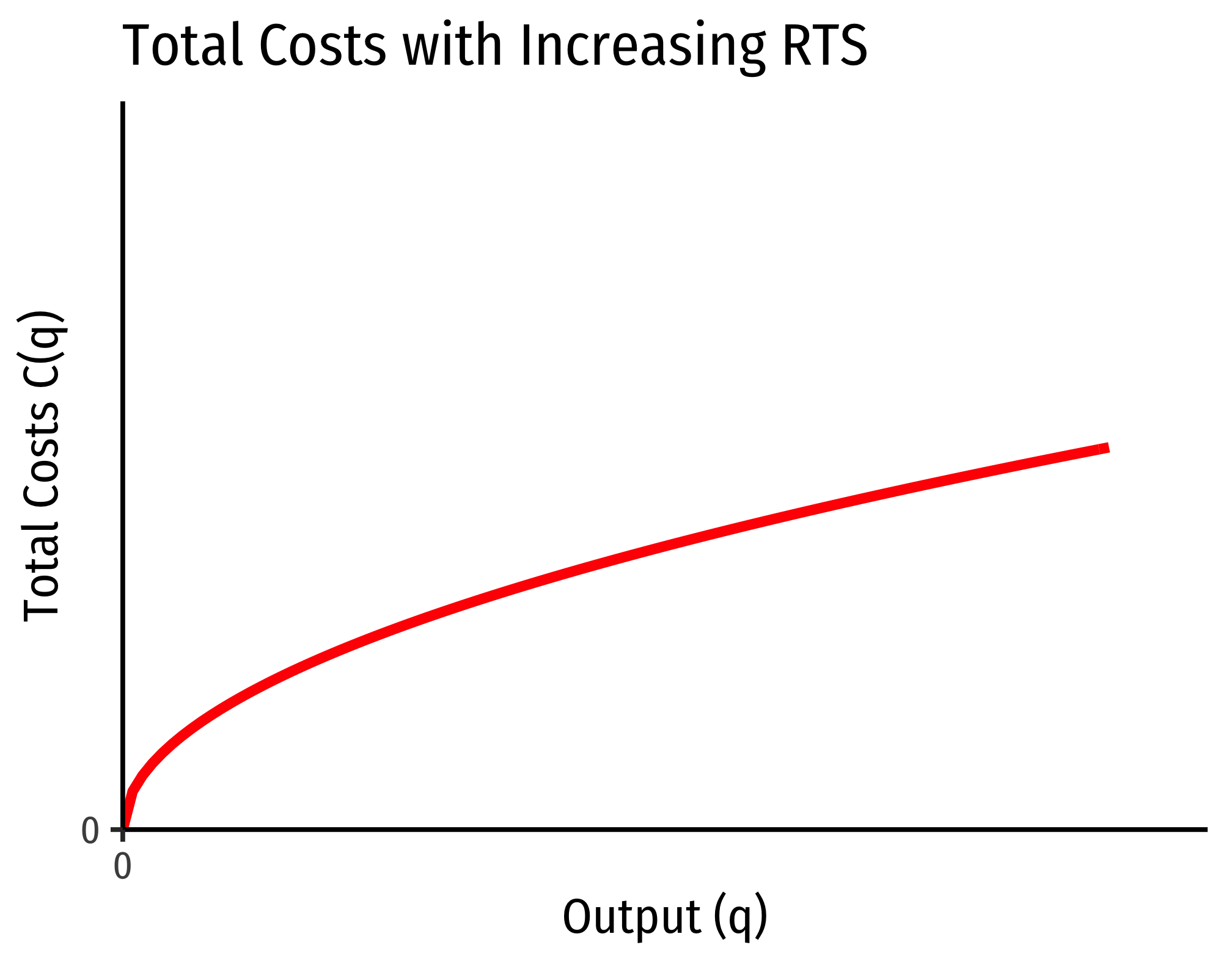
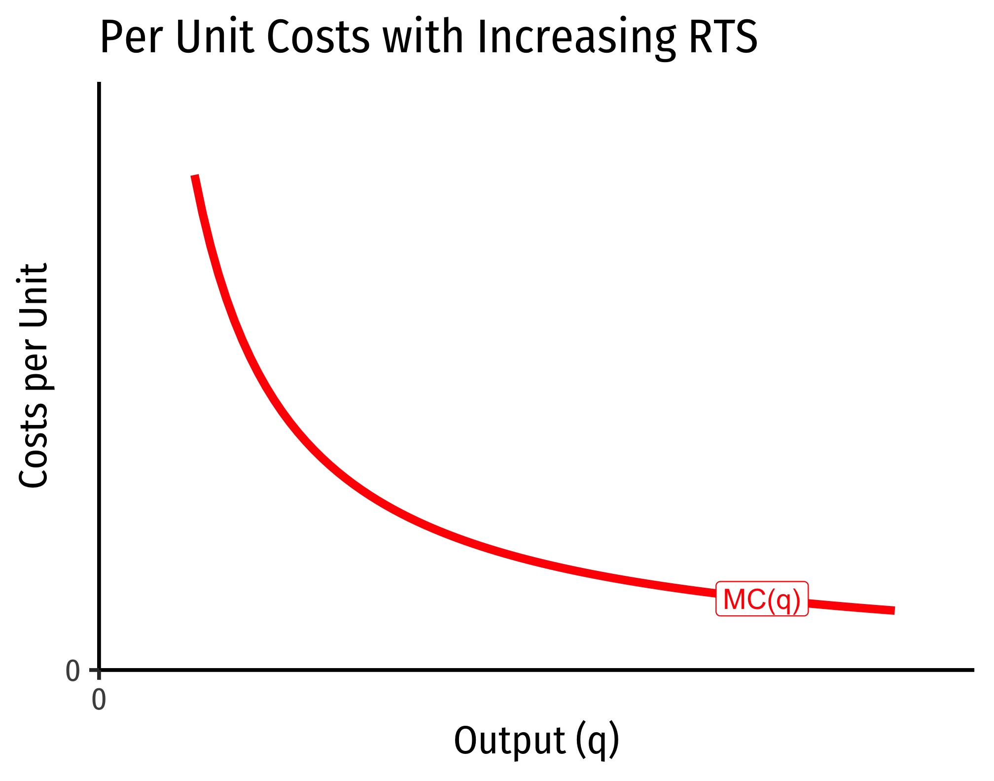
Increasing Returns to Scale
Cobb-Douglas Cost Functions
The total cost function for Cobb-Douglas production functions of the form \[q=l^{\alpha}k^{\beta}\] can be shown with some very tedious algebra to be:
\[C(w,r,q)=\left[\left(\frac{\alpha}{\beta}\right)^{\frac{\beta}{\alpha+\beta}} + \left(\frac{\alpha}{\beta}\right)^{\frac{-\alpha}{\alpha+\beta}}\right] w^{\frac{\alpha}{\alpha+\beta}} r^{\frac{\beta}{\alpha+\beta}} q^{\frac{1}{\alpha+\beta}}\]
If you take the first derivative of this (to get marginal cost), it is:
\[\frac{\partial C(w,r,q)}{\partial q}= MC(q) = \frac{1}{\alpha+\beta} \left(w^{\frac{\alpha}{\alpha+\beta}} r^{\frac{\beta}{\alpha+\beta}}\right) q^{\left(\frac{1}{\alpha+\beta}\right)-1}\]
How does marginal cost change with increased output? Take the second derivative:
\[\frac{\partial^2 C(w,r,q)}{\partial q^2}= \frac{1}{\alpha+\beta} \left(\frac{1}{\alpha+\beta} -1 \right) \left(w^{\frac{\alpha}{\alpha+\beta}} r^{\frac{\beta}{\alpha+\beta}}\right) q^{\left(\frac{1}{\alpha+\beta}\right)-2}\]
- If \(\frac{1}{\alpha+\beta} > 1\), this is positive \(\implies\) decreasing returns to scale
- \(\alpha+\beta < 1\) in the production function
- If \(\frac{1}{\alpha+\beta} < 1\), this is negative \(\implies\) increasing returns to scale
- \(\alpha+\beta > 1\) in the production function
- If \(\frac{1}{\alpha+\beta} = 1\), this is constant \(\implies\) constant returns to scale
- \(\alpha+\beta = 1\) in the production function
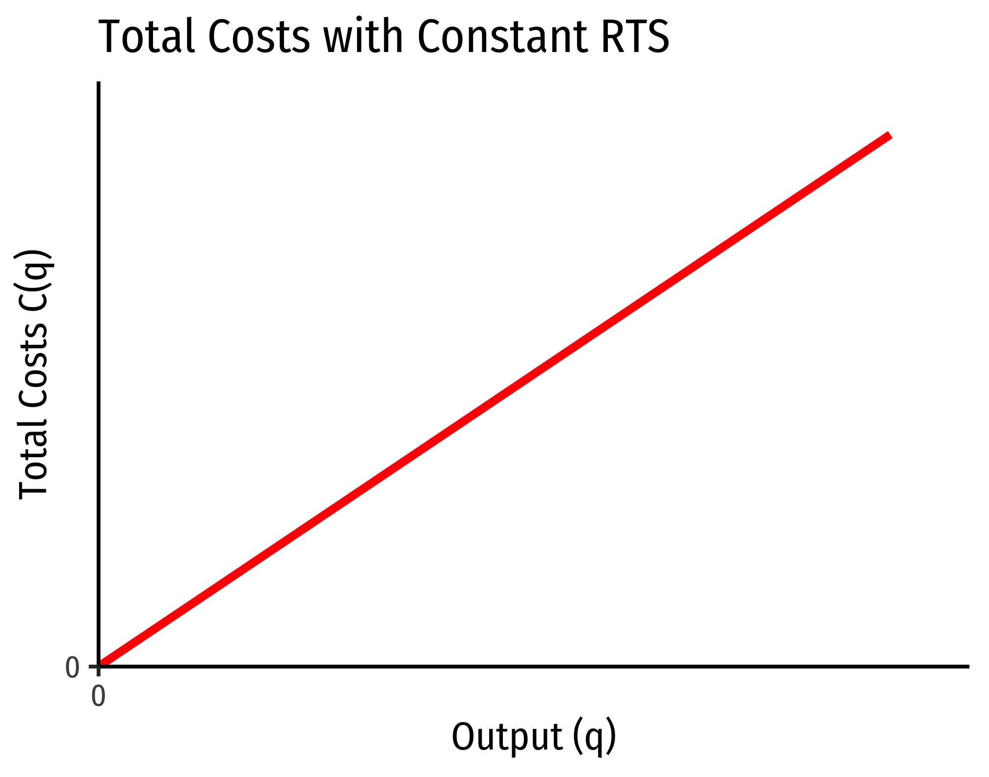
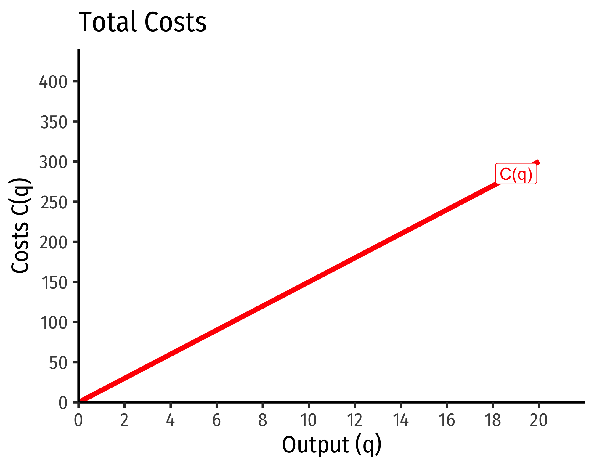
Example (Constant Returns)
Let \(q=l^{0.5}k^{0.5}\).
\[\begin{align*} C(w,r,q)&=\left[\left(\frac{0.5}{0.5}\right)^{\frac{0.5}{0.5+0.5}} + \left(\frac{0.5}{0.5}\right)^{\frac{-0.5}{0.5+0.5}}\right] w^{\frac{0.5}{0.5+0.5}} r^{\frac{0.5}{0.5+0.5}} q^{\frac{1}{0.5+0.5}}\\ C(w,r,q)&= \left[1^{0.5}+1^{-0.5} \right]w^{0.5}r^{0.5}q^{0.5}\\ C(w,r,q)&= w^{0.5}r^{0.5}q^{1}\\ \end{align*}\]
If \(w=9\), \(r=25\):
\[\begin{align*}C(w=10,r=20,q)&=9^{0.5}25^{0.5}q \\ & =3*5*q\\ & =15q\\\end{align*}\]
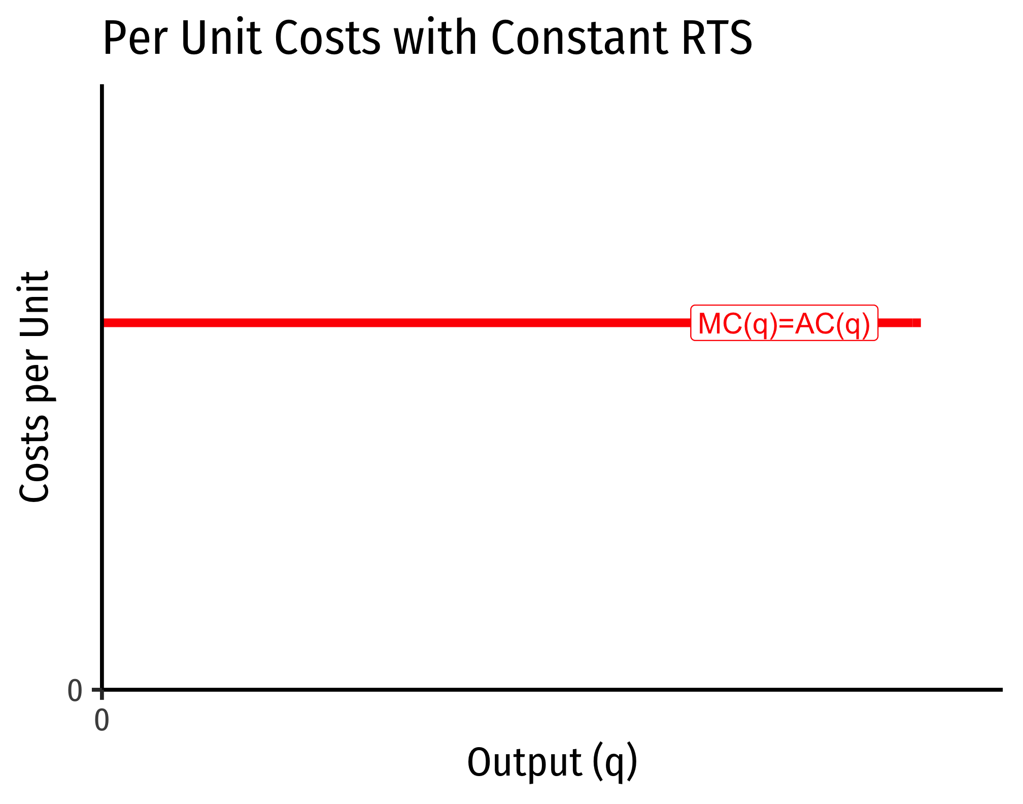
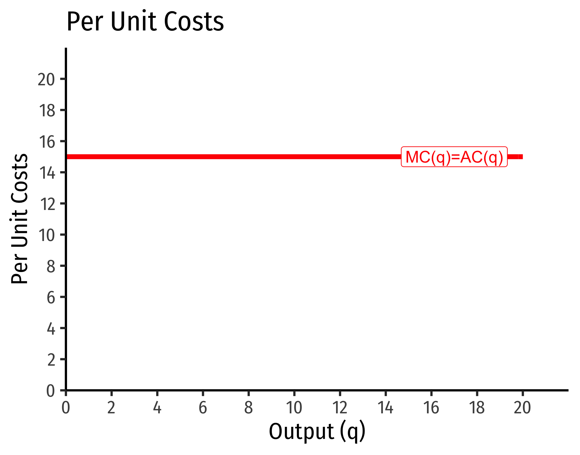
Marginal costs would be
\[MC(q) = \frac{\partial C(q)}{\partial q} = 15\]
Average costs would be
\[MC(q) = \frac{C(q)}{q} = \frac{15q}{q} = 15\]
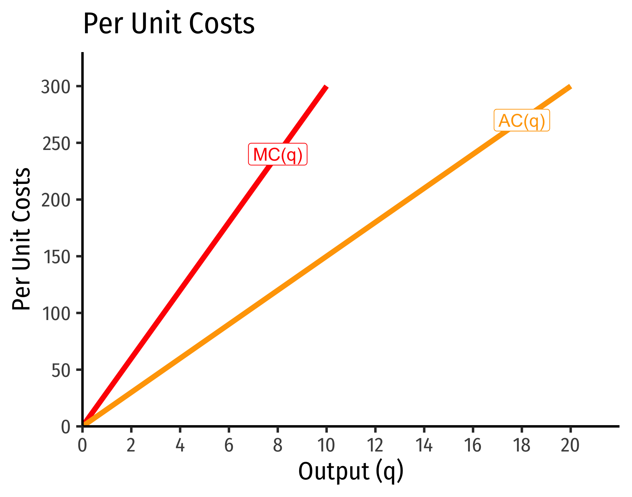
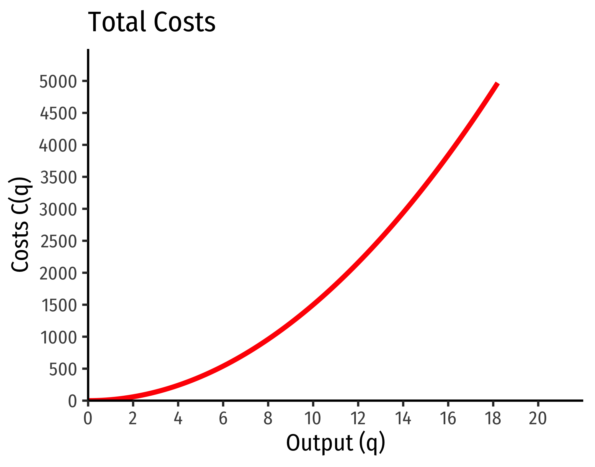
Example (Decreasing Returns)
Let \(q=l^{0.25}k^{0.25}\).
\[\begin{align*} C(w,r,q)&=\left[\left(\frac{0.25}{0.25}\right)^{\frac{0.25}{0.25+0.25}} + \left(\frac{0.25}{0.25}\right)^{\frac{-0.25}{0.25+0.25}}\right] w^{\frac{0.25}{0.25+0.25}} r^{\frac{0.25}{0.25+0.25}} q^{\frac{1}{0.25+0.25}}\\ C(w,r,q)&= \left[1^{0.5}+1^{-0.5} \right]w^{0.5}r^{0.5}q^{2}\\ C(w,r,q)&= w^{0.5}r^{0.5}q^{2}\\ \end{align*}\]
If \(w=9\), \(r=25\):
\[\begin{align*}C(w=10,r=20,q)&=9^{0.5}25^{0.5}q^2 \\ & =3*5*q^2\\ & =15q^2\\\end{align*}\]
Marginal costs would be
\[MC(q) = \frac{\partial C(q)}{\partial q} = 30q\]
Average costs would be
\[AC(q) = \frac{C(q)}{q} = \frac{15q^2}{q} = 15q\]