The Consumer's Problem: Review
- The consumer's constrained optimization problem is:
Choose: < a consumption bundle >
In order to maximize: < utility >
Subject to: < income and market prices >

The Consumer's Problem: Tools
We now have the tools to understand consumer choices:
Budget constraint: consumer's constraints of income and market prices
- How the .red[market] trades off between two goods
- Utility function: consumer's preferences to maximize
- How the .green[consumer] trades off between two goods
The Consumer's Problem: Verbally
- The consumer's constrained optimization problem:
choose a bundle of goods to maximize utility, subject to income and market prices
The Consumer's Problem: Mathematically
maxx,yu(x,y)
- This requires calculus to solve1. We will look at graphs instead!
1 See the mathematical appendix in today's class notes on how to solve it with calculus, and an example.
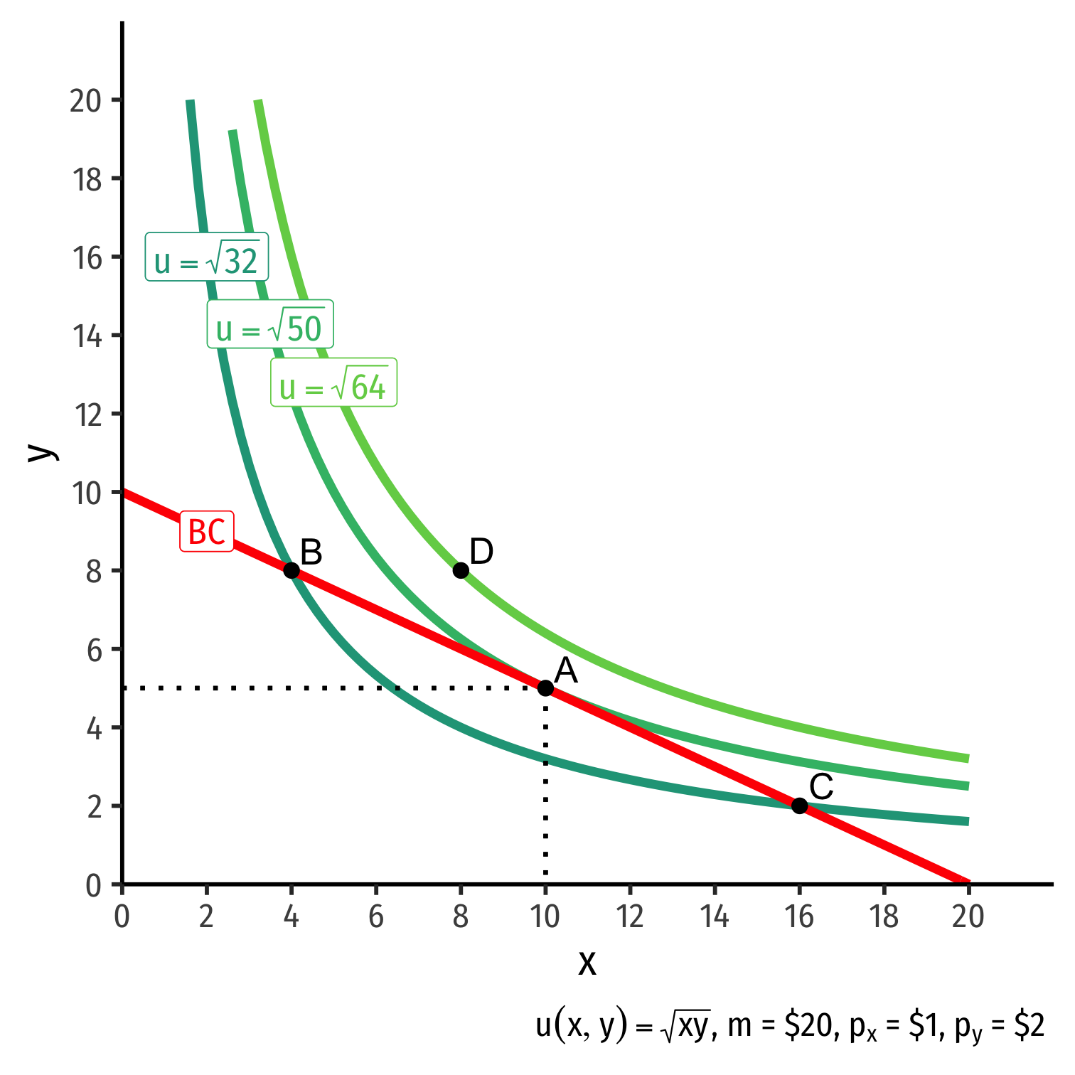
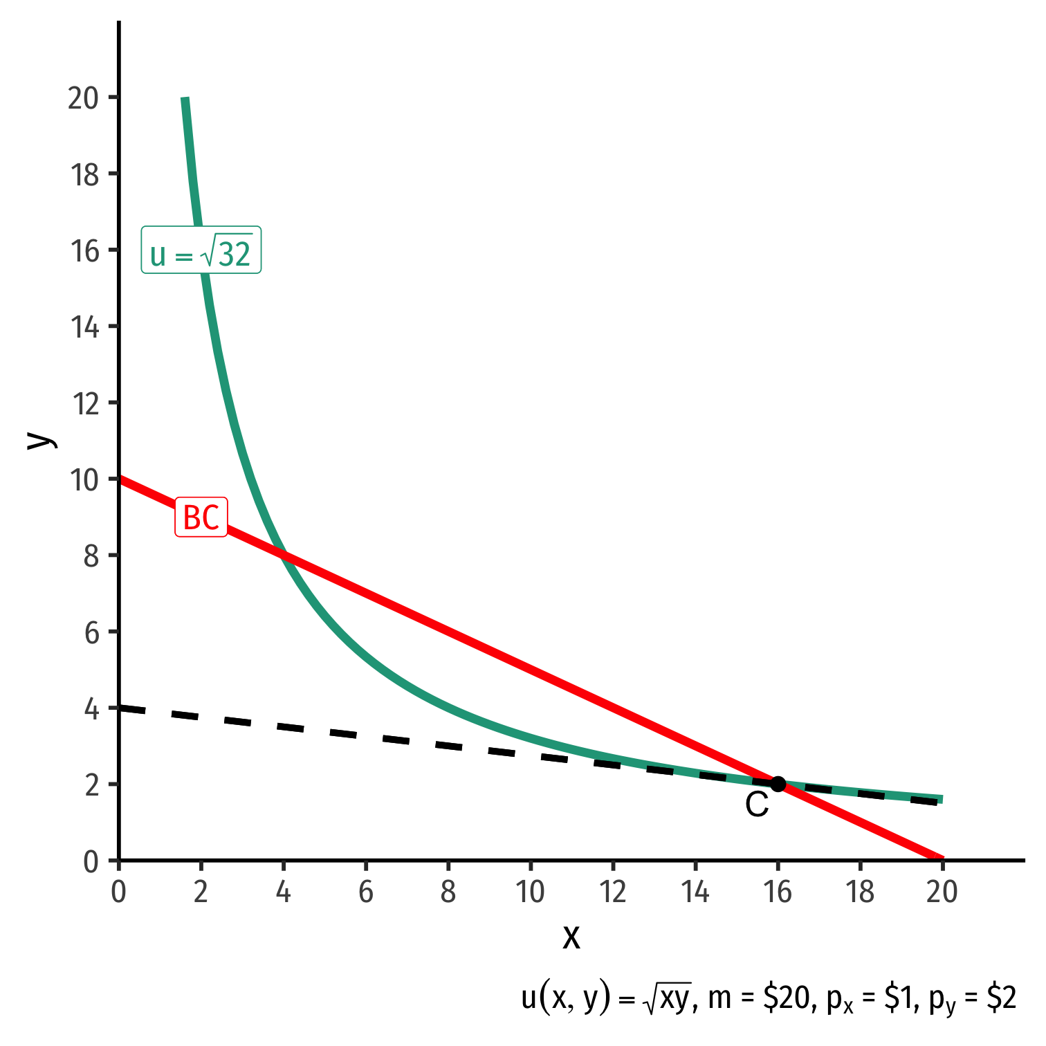
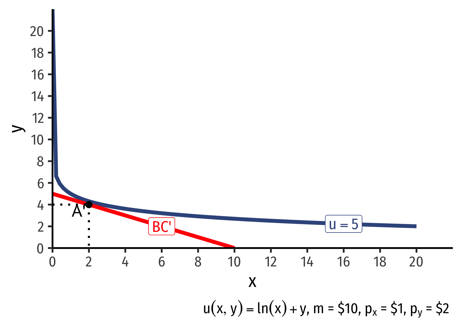
The Consumer's Optimum: Graphically
- Graphical solution: Highest indifference curve tangent to budget constraint
- Bundle A!
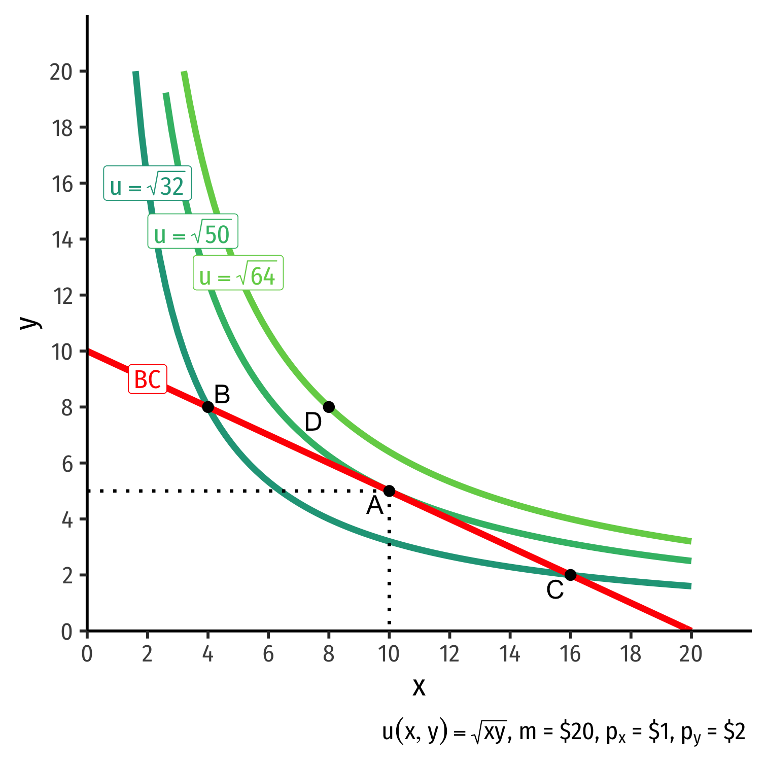
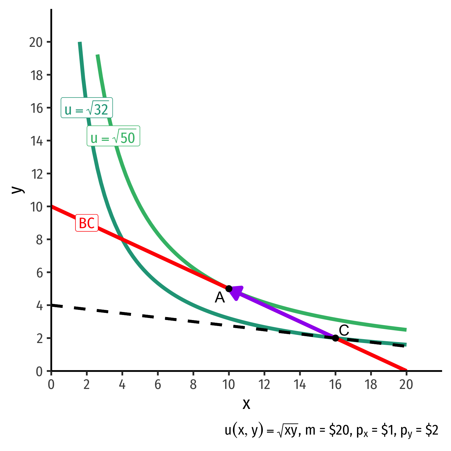
The Consumer's Optimum: Graphically
Graphical solution: Highest indifference curve tangent to budget constraint
- Bundle A!
B or C spend all income, but a better combination exists
- Averages ≻ extremes!

The Consumer's Optimum: Graphically
Graphical solution: Highest indifference curve tangent to budget constraint
- Bundle A!
B or C spend all income, but a better combination exists
- Averages ≻ extremes!
D is higher utility, but not affordable at current income & prices
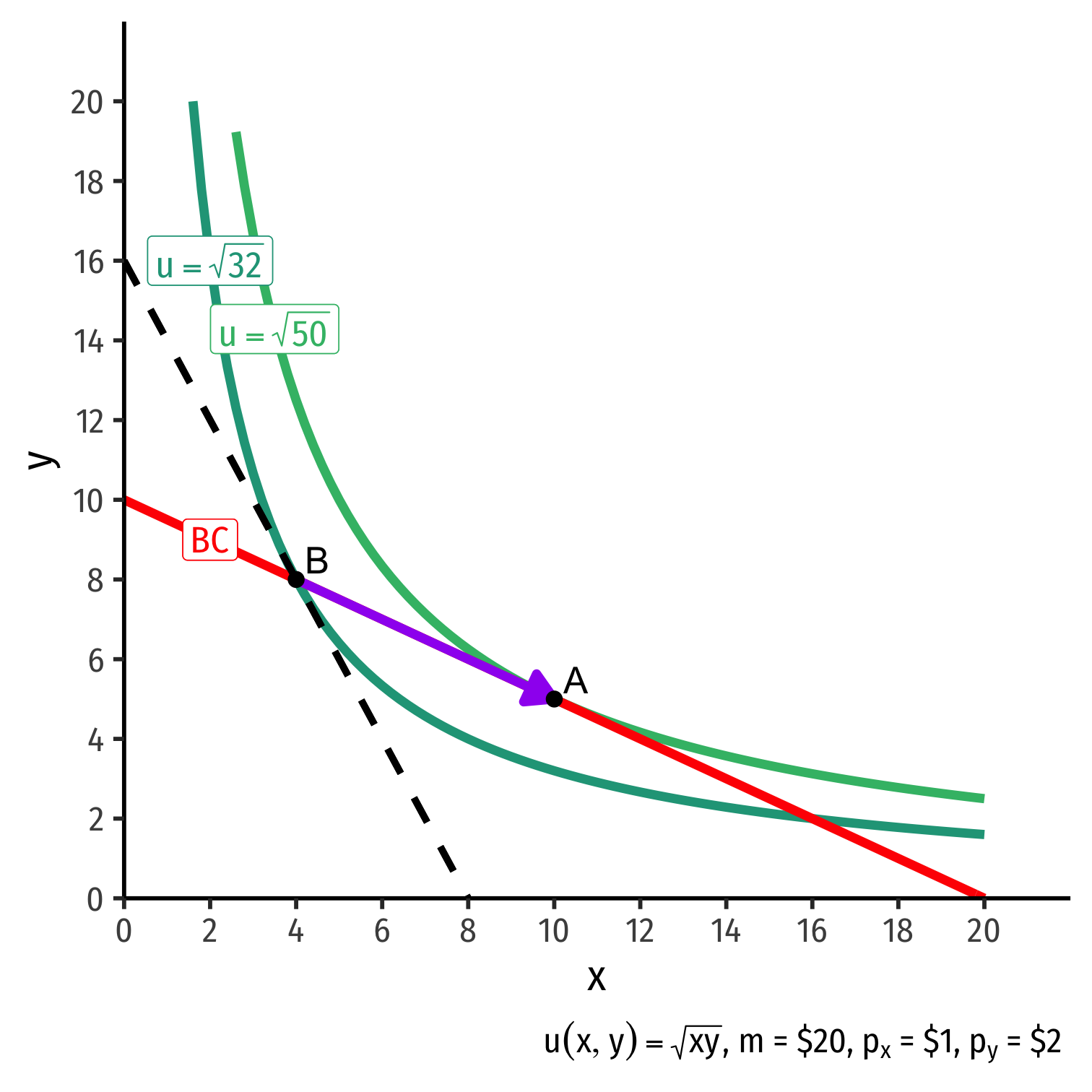
The Consumer's Optimum: Why Not B?
indiff. curve slope>budget constr. slope
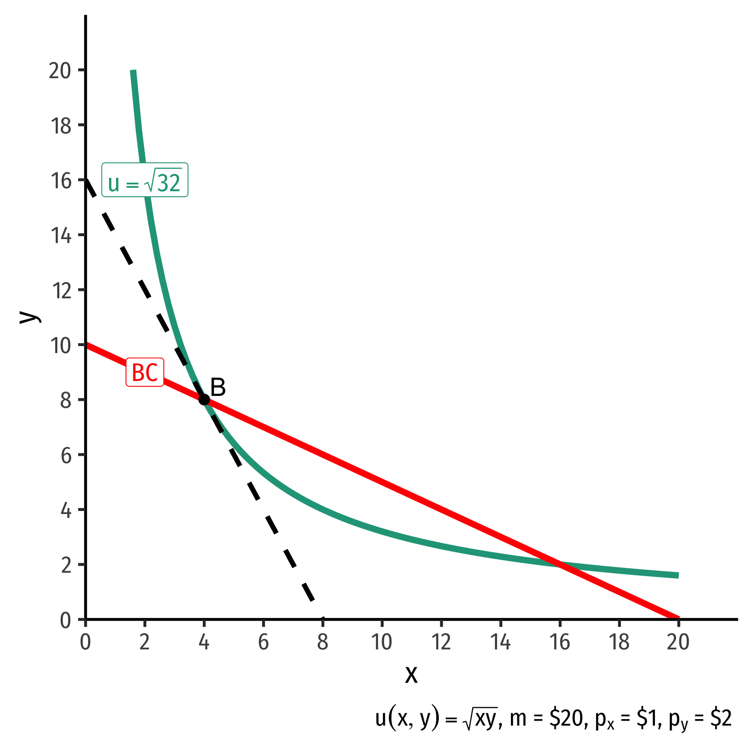
The Consumer's Optimum: Why Not B?
indiff. curve slope>budget constr. slope|MRSx,y|>|pxpy||MUxMUy|>|pxpy||−2|>|−0.5|
Consumer would exchange at 2Y:1X
Market exchange rate is 0.5Y:1X

The Consumer's Optimum: Why Not B?
indiff. curve slope>budget constr. slope|MRSx,y|>|pxpy||MUxMUy|>|pxpy||−2|>|−0.5|
Consumer would exchange at 2Y:1X
Market exchange rate is 0.5Y:1X
Can spend less on y more on x and get more utility!
The Consumer's Optimum: Why Not C?
indiff. curve slope<budget constr. slope
The Consumer's Optimum: Why Not C?
indiff. curve slope<budget constr. slope|MRSx,y|<|pxpy||MUxMUy|<|pxpy||−0.125|<|−0.5|
Consumer would exchange at 0.125Y:1X
Market exchange rate is 0.5Y:1X

The Consumer's Optimum: Why Not C?
indiff. curve slope<budget constr. slope|MRSx,y|<|pxpy||MUxMUy|<|pxpy||−0.125|<|−0.5|
Consumer would exchange at 0.125Y:1X
Market exchange rate is 0.5Y:1X
Can spend less on x, more on y and get more utility!
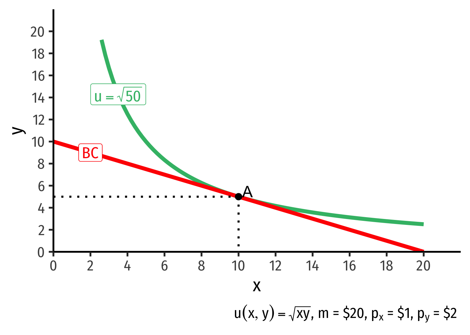
The Consumer's Optimum: Why A?
indiff. curve slope=budget constr. slope
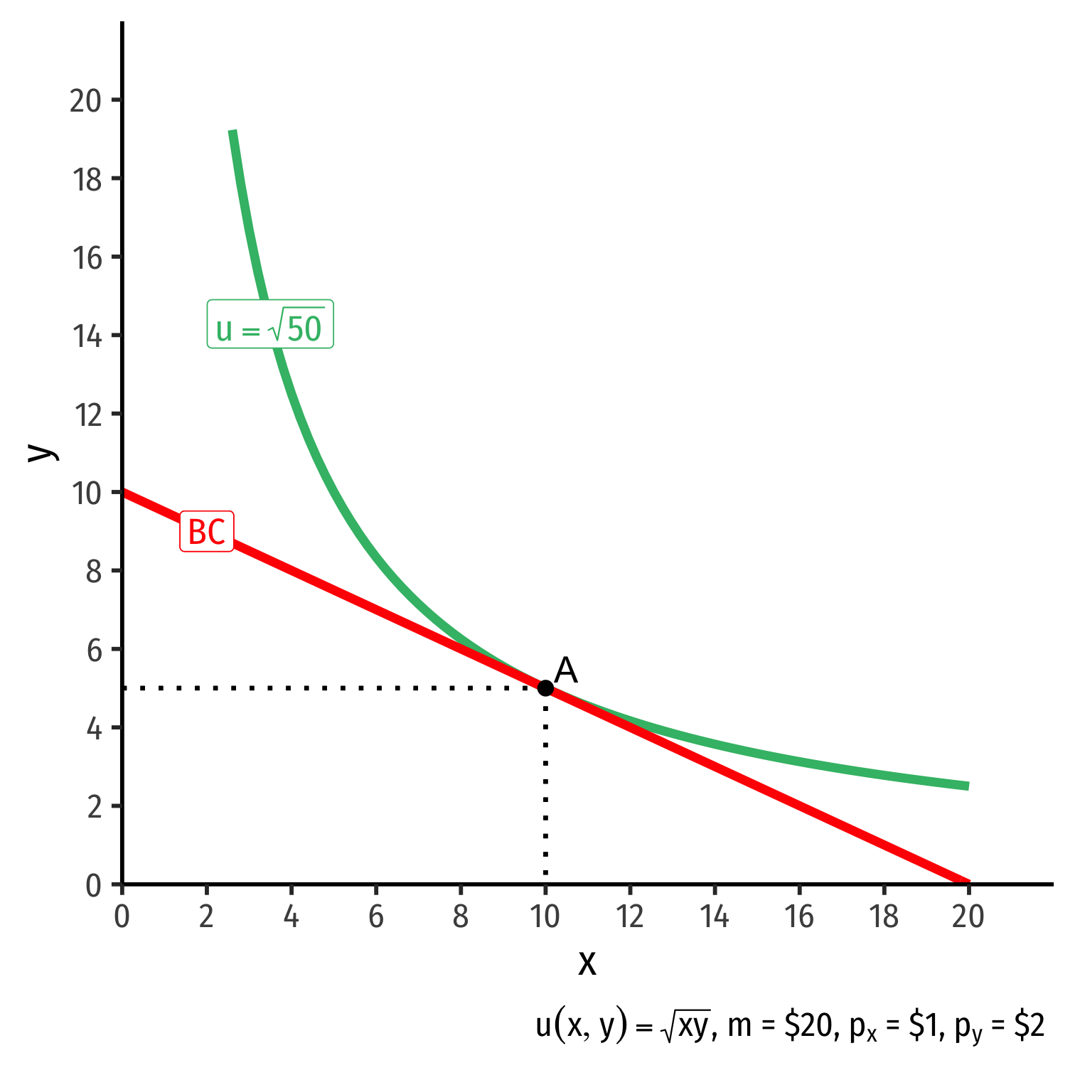
The Consumer's Optimum: Why A?
indiff. curve slope=budget constr. slope|MRSx,y|=|pxpy||MUxMUy|=|pxpy||−0.5|=|−0.5|
Consumer would exchange at same rate as market
No other combination of (x,y) exists at current prices & income that could increase utility!

The Consumer's Optimum: Two Equivalent Rules
Rule 1
MUxMUy=pxpy
- Easier for solving math problems (slope of each curve)

The Consumer's Optimum: Two Equivalent Rules
Rule 1
MUxMUy=pxpy
- Easier for calculation (slopes)
Rule 2
MUxpx=MUypy
- Easier for intuition (next slide)

The Consumer's Optimum: The Equimarginal Rule III
Any optimum in economics: no better alternatives exist under current constraints
No possible change in your consumption that would increase your utility

Markets Equalize Everyone's MRS I
Markets make it so everyone faces the same relative prices
- Budget constraint. slope, −pxpy
- Note individuals' incomes, m, are certainly different!
A person's optimal choice ⟹ they make same tradeoff as the market
- Their MRS = relative price ratio
markets equalize everyone's MRS

Markets Equalize Everyone's MRS II
Two people will very different income and preferences face the same market prices, and choose optimal consumption (points A and A') at an exchange rate of 0.5Y:1X
Optimization and Equilibrium
If people can learn and change their behavior, they will always switch to a higher-valued option
If a person has no better choices (under current constraints), they are at an optimum
If everyone is at an optimum, the system is in equilibrium