The Consumer's Problem: Review
We now can explore the dynamics of how consumers optimally respond to changes in their constraints
We know the problem is:
Choose: < a consumption bundle >
In order to maximize: < utility >
Subject to: < income and market prices >

A Demand Function (for Good X)
- A consumer's demand (for good x) depends on current prices & income:
qDx=qDx(m,px,py)
- How does demand for x change?
A Demand Function (for Good X)
- A consumer's demand (for good x) depends on current prices & income:
qDx=qDx(m,px,py)
- How does demand for x change?
- Income effects (ΔqDxΔm): how qDx changes with changes in income
A Demand Function (for Good X)
- A consumer's demand (for good x) depends on current prices & income:
qDx=qDx(m,px,py)
- How does demand for x change?
- Income effects (ΔqDxΔm): how qDx changes with changes in income
- Cross-price effects (ΔqDxΔpy): how qDx changes with changes in prices of other goods (e.g. y)
- (Own) Price effects (ΔqDxΔpx): how qDx changes with changes in price (of x)
Income Effect
- Income effect: change in optimal consumption of a good associated with a change in (nominal) income, holding relative prices constant
ΔqDΔm>?<0

Income Effect (Normal)
- Consider football tickets and vacation days
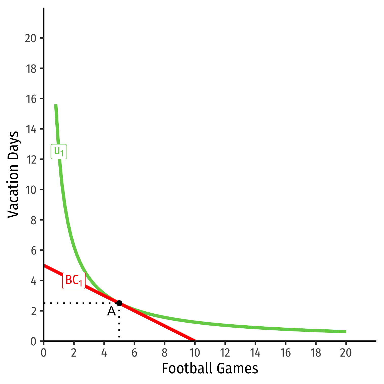
Income Effect (Normal)
Consider football tickets and vacation days
Suppose income (m) increases
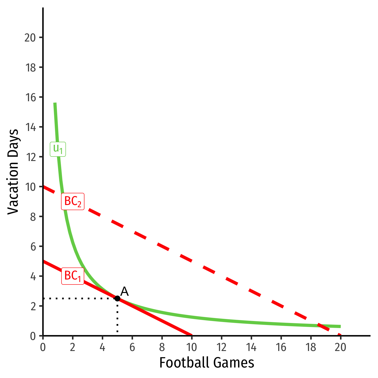
Income Effect (Normal)
Consider football tickets and vacation days
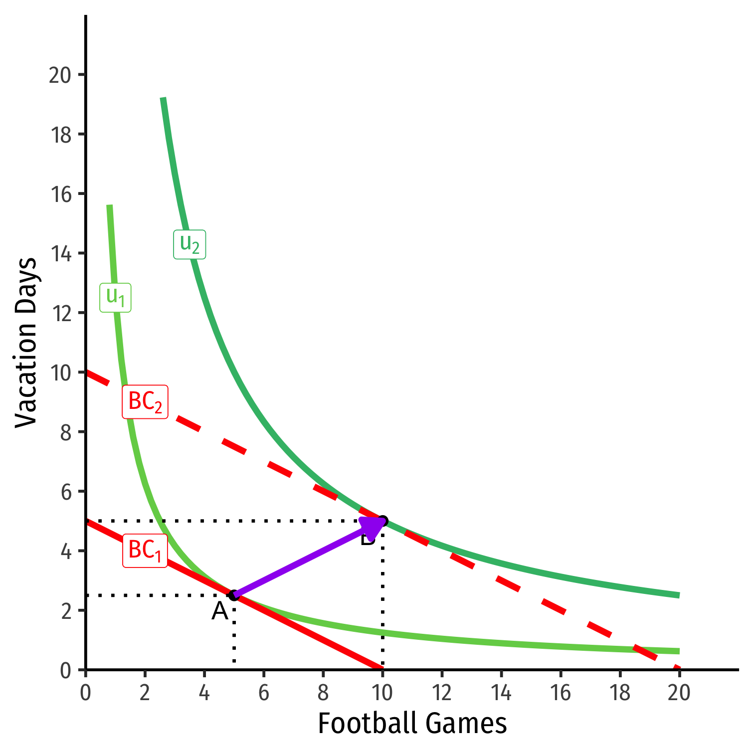
Suppose income (m) increases
At new optimum (B), consumes more of both
Then both goods are normal goods
Income Effect (Inferior)
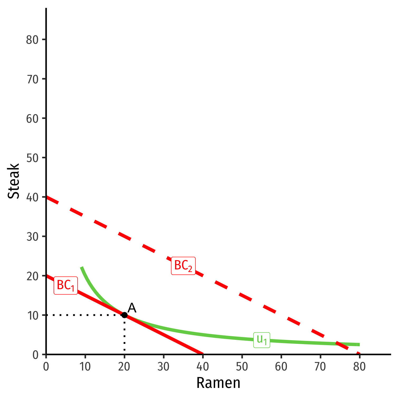
- Consider ramen and steak
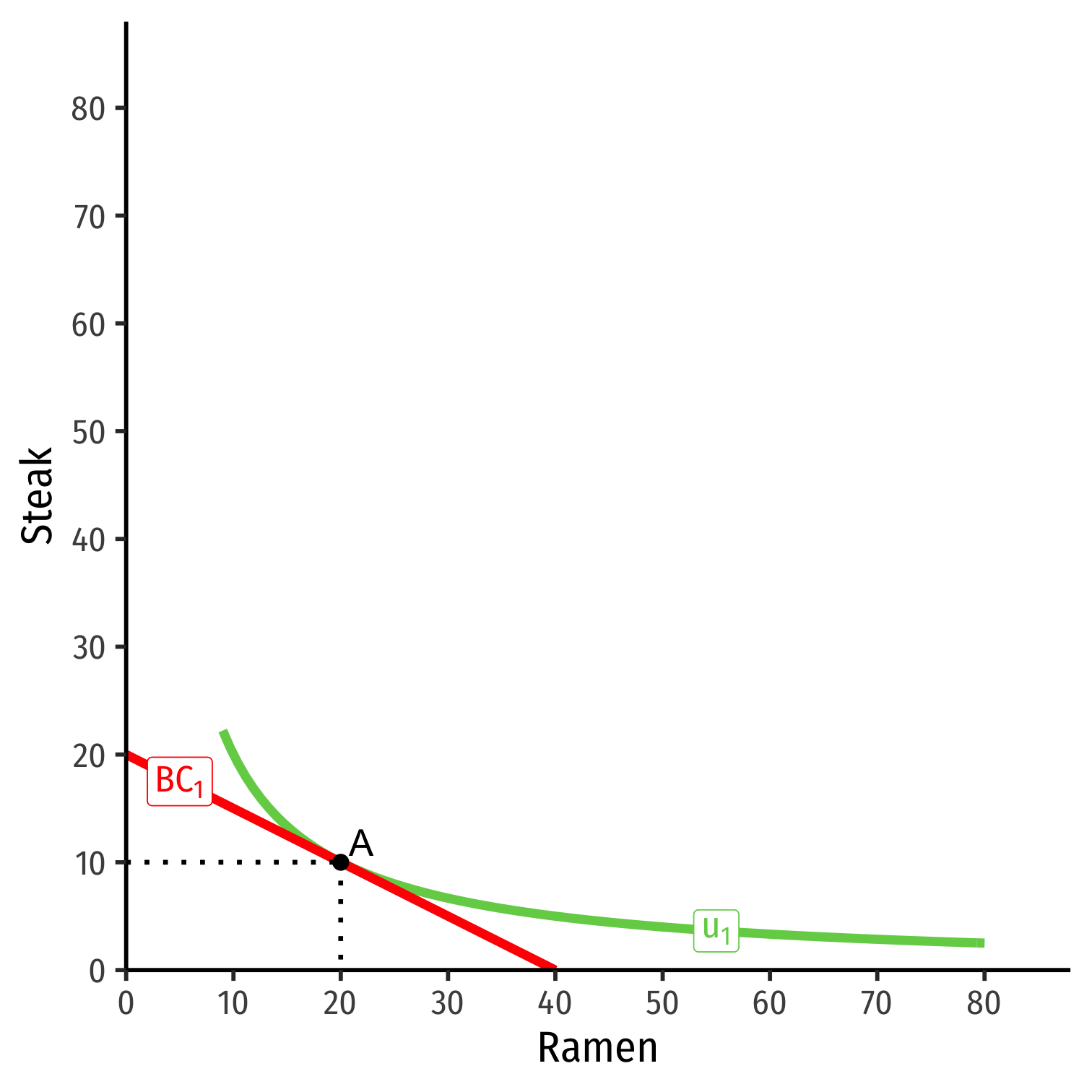
Income Effect (Inferior)
Consider ramen and steak
Suppose income (m) increases
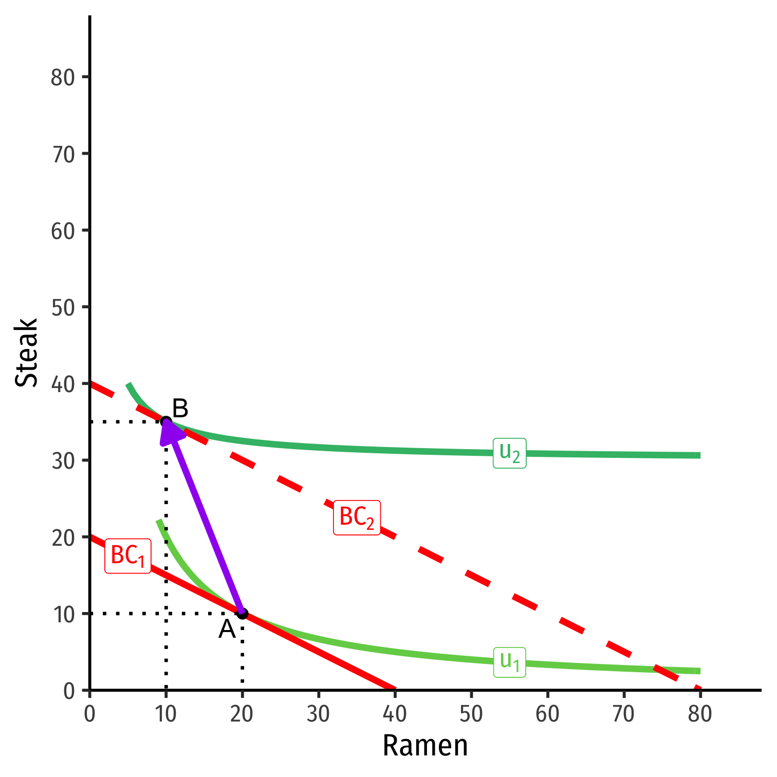
Income Effect (Inferior)
Consider ramen and steak
Suppose income (m) increases
At new optimum (B), consumes more steak, less ramen
Steak is a normal good, ramen is an inferior good
Income Effect
ΔqDΔm>?<0
Normal goods: consumption increases with more income (and vice versa)
Inferior goods: consumption decreases with more income (and vice versa)
Income Effects: Example
Example: Is the environment a normal good?

Income Effects: Example
Example: Is the environment a normal good?

Income Expansion Path

Goolsbee, et. al (2011: 169)
- Income expansion path describes how consumption of each good changes when income increases
- Traces a line between optimal consumption points as income increases (budget constraint shifts out)
Engel Curves

Goolsbee, et. al (2011: 171)
- Engel curve of each good is more helpful to visualize: shows how consumption of one good changes when income increases
Cross-Price Effects
- Cross-price effect: change in optimal consumption of a good associated with a change in price of another good income, holding the good's own price (and income) constant
ΔqxΔpy>?<0

Cross-Price Elasticity of Demand I
- The cross-price elasticity of demand measures how much quantity demanded of one good (qx) changes in response to a change in price of another good (py)
ϵqx,py=%Δqx%Δpy
Cross-Price Elasticity of Demand I
- The cross-price elasticity of demand measures how much quantity demanded of one good (qx) changes in response to a change in price of another good (py)
ϵqx,py=%Δqx%Δpy=ΔqxqxΔpypy
Cross-Price Elasticity of Demand II
ϵqx,py=%Δqx%Δpy
If ϵqx,py is positive: goods x and y are substitutes
An rise (fall) in price of y causes more (less) consumption of x
- Consumption of x moves in same direction as price of y

Cross-Price Elasticity of Demand III
ϵqx,py=%Δqx%Δpy
If ϵqx,py is negative: goods x and y are complements
Goods x and y consumed in a bundle, concern about overall price of bundle
A rise (fall) in price of y causes less (more) consumption of x
- Consumption of x moves in opposite direction as price of y
